Big Game Meets BigQuery – Super Bowl XLIX Prediction

It’s that time of year again. Super Bowl XLIX is upon us, and it has the makings of a great one. The Valley of the Sun (Glendale, Arizona) will host this meeting between the #1 seeds from both football conferences. The Patriots romped through the AFC championship, disposing of the Colts 45-7 (perhaps with the help of some deflated footballs), while the Seahawks were pushed to the brink by Green Bay in one of the best NFC title games in recent memory.

In this post, we’re going to make an audacious prediction for this year’s game by:

1. Downloading team data from the ESPN public dataset
2. Uploading that data into BigQuery
3. Running queries on the data within BigQuery

Downloading Team Data from ESPN

As the first step, we head to http://espn.go.com/nfl/statistics to download data for the 2014 Regular Season as three CSV files: offense.csv, defense.csv, and specialteams.csv.

Thank you, ESPN. 🙂

Finding the data is the easy part. There are veritable oceans of football data available, most of which I felt would complicate the purpose of this post, so I settled on using some basic, easy-to-understand stats.

Uploading into BigQuery

Once it’s collected, how should we analyze the data? Excel? Tableau? Or perhaps something a little, shall we say, BIGger… We’re talking about a BIG game after all.

Although we could pull the downloaded data into any number of DBMSs, spreadsheet programs, or visualization tools, I figured that the Super Bowl prediction would be a great way to illustrate the process of importing data into BigQuery, and then showcase some of BigQuery’s many data slicing and analytical features.

There are a few ways of loading data into BigQuery:

• stream the data into BigQuery programmatically
• load the data from Google Cloud Storage
• upload small data sets via CSV/JSON files

For the purpose of this discussion, we will focus on the third method (CSV/JSON) only. (We already have the CSV files downloaded from ESPN and ready to go.)

Uploading data into BigQuery via this method is fairly straightforward:

1. Create a dataset: Create a dataset by selecting the arrow next to your project and clicking on Create new dataset. For this example, we will call our dataset superbowl2015.
   
2. Create tables within the dataset: To do this, click the dropdown arrow next to the dataset and select Create new table. We’ll call the table offense (and perform all the same steps for two more tables, defense and specialteams).
   
3. Load data into the tables: After doing all the steps above, clicking the submit button will load the data into the table(s) we created. Based on the size of the data, the upload can take seconds or minutes. Watch out for error messages indicated by a red exclamation mark.
4. Upload data into the tables:
   • Choose destination: offense.
   • Choose data: we’ll select the offense.csv file that we downloaded previously.
   • Specify schema: this is a little bit of a manual process. We will need to specify a data type for each column of the CSV file as in the following example (where yards_g means yards per game):
     Team:String,Yards:integer,Yards_g:float
   • Specify advanced options: optionally configure field delimiters, header rows to skip, and error handling.
   • Submit: wait a moment, and your CSV data should now be fully uploaded into your new BigQuery table.

Create the offense table within the dataset, and import data into the table.

Select the data source format, and browse for the file.

Specify the data type for each column in the CSV file.
Actual schema used: TEAM:string,YDS:integer,YDS_G,float,PASS:integer,P_YDS_G:float,RUSH:integer,R_YDS_G:float,PTS:integer,PTS_G:float

Table Schemas

What kind of data do we now have to work with? Below are the schemas for our three tables.

Field	Type	Description
Team	String	Name of Team
Yds	Integer	Yards
Yds_G	Float	Yards per Game
Pass	Integer	Passing Yards
P_Yds_G	Float	Passing Yards per Game
Rush	Integer	Rushing Yards
R_Yds_G	Float	Rushing Yards per Game
Pts	Integer	Points
Pts_G	Float	Points per game

Field	Type	Description
Team	String	Name of Team
Yds	Integer	Yards
Yds_G	Float	Yards per Game
Pass	Integer	Passing Yards
P_Yds_G	Float	Passing Yards per Game
Rush	Integer	Rushing Yards
R_Yds_G	Float	Rushing Yards per Game
Pts	Integer	Points
Pts_G	Float	Points per game

Field	Type	Description
Team	String	Name of Team
Fgm	Integer	Field Goals Made
Fga	Integer	Field Goals Against

 

On to the fun stuff 🙂

Querying in BigQuery

The concept behind this prediction is to rank each team (Patriots and Seahawks) by evaluating all stats for each team in offensive, defensive and special teams categories. Once we know the rank in each category, it’s just a matter of totaling the score and seeing who comes out ahead.

Let’s start with a simple query just to make sure it works. The following query will show us the top 9 teams in the league by total yards.

SELECT team,yds FROM [superbowl2015.offense] order by yds DESC LIMIT 1000

Now that we’ve established that we can query the data that we just uploaded, we will determine the rank of each team in all stats for the offense category/table. We will do this by checking each column in the Offense table and determine where each team ranks respectively. Luckily BigQuery has support for analytical functions such as rank, percentiles, relative row navigation, etc. Using the powerful rank command, we come up with the following query:

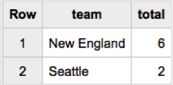
SELECT team,
rank() OVER (ORDER BY yds DESC) rk_yds,
rank() OVER (ORDER BY yds_g DESC) rk_yds_g,
rank() OVER (ORDER BY pass DESC) rk_pass,
rank() OVER (ORDER BY pass DESC) rk_p_yds_g,
rank() OVER (ORDER BY pass DESC) rk_rush,
rank() OVER (ORDER BY pass DESC) rk_r_yds_g,
rank() OVER (ORDER BY pass DESC) rk_pts,
rank() OVER (ORDER BY pass DESC) rk_pts_g,
FROM [superbowl2015.offense] WHERE
   team='Seattle' or team='New England' LIMIT 1000 

This query produced the following results:

This quickly shows us that New England is ranked higher in more offensive stats (6) than Seattle (2). Let’s take this one step further though because I don’t want to have to add this up each time. I would rather BigQuery do this for me. It should be possible to add the values across rows (as opposed to summing columns) right?

The queries below leverage the case function to evaluate the results of the nested select statement. Each query essentially counts all the values in each row where the team is ranked as #1. (It should be noted, that there may, in some circumstances, be more optimal ways of summing the row values then what is shown below. This method was just a quick and simple approach for the dataset being used.)

Querying for Offense

select team,sum
(case when rk_yds=1 then 1 else 0 end)+sum(case when rk_yds_g=1 then 1 else 0 end)
+sum(case when rk_pass=1 then 1 else 0 end)+sum(case when rk_p_yds_g=1 then 1 else 0 end)
+sum(case when rk_rush=1 then 1 else 0 end)+sum(case when rk_r_yds_g=1 then 1 else 0 end)
+sum(case when rk_pts=1 then 1 else 0 end)+sum(case when rk_pts_g=1 then 1 else 0 end) as total from 
(SELECT team,
rank() OVER (ORDER BY yds DESC) rk_yds,
rank() OVER (ORDER BY yds_g DESC) rk_yds_g,
rank() OVER (ORDER BY pass DESC) rk_pass,
rank() OVER (ORDER BY pass DESC) rk_p_yds_g,
rank() OVER (ORDER BY pass DESC) rk_rush,
rank() OVER (ORDER BY pass DESC) rk_r_yds_g,
rank() OVER (ORDER BY pass DESC) rk_pts,
rank() OVER (ORDER BY pass DESC) rk_pts_g,
FROM [superbowl2015.offense] WHERE
   team='Seattle' or team='New England' LIMIT 1000 ) group by team.

Looks a little intimidating, but it’s not that complex once you break down all the elements. Using this query, we end up with:

Offense – Winner: New England

Much better. 🙂

The data clearly shows that New England has the better offensive team. The Patriots had one of the best offenses in the regular season, while Seattle didn’t find their rhythm until later in the year. Tom Brady and the Patriots will give Seattle all they can handle.

Let’s apply the same concept to the other two categories.

Querying for Defense

select team,sum
(case when rk_yds=1 then 1 else 0 end)+sum(case when rk_yds_g=1 then 1 else 0 end)
+sum(case when rk_pass=1 then 1 else 0 end)+sum(case when rk_p_yds_g=1 then 1 else 0 end)
+sum(case when rk_rush=1 then 1 else 0 end)+sum(case when rk_r_yds_g=1 then 1 else 0 end)
+sum(case when rk_pts=1 then 1 else 0 end)+sum(case when rk_pts_g=1 then 1 else 0 end) as total from 
(SELECT team,
rank() OVER (ORDER BY yds DESC) rk_yds,
rank() OVER (ORDER BY yds_g DESC) rk_yds_g,
rank() OVER (ORDER BY pass DESC) rk_pass,
rank() OVER (ORDER BY pass DESC) rk_p_yds_g,
rank() OVER (ORDER BY pass DESC) rk_rush,
rank() OVER (ORDER BY pass DESC) rk_r_yds_g,
rank() OVER (ORDER BY pass DESC) rk_pts,
rank() OVER (ORDER BY pass DESC) rk_pts_g,
FROM [superbowl2015.offense] WHERE
   team='Seattle' or team='New England' LIMIT 1000 ) group by team.

Defense – Winner: Seattle

Wow! I knew without even looking at the data that Seattle had a better defense, but I didn’t expect them to win this category so convincingly. What a matchup this will be! Keep in mind that I had to reverse the rank in this scenario, since the goal of playing well defensively is to allow the least yards, points, etc.

Querying for Special Teams

select team,sum(case when rk_fgm=1 then 1 else 0 end)+sum(case when rk_fga=1 then 1 else 0 end)
 as total from 
(SELECT team,
rank() OVER (ORDER BY fgm ASC) rk_fgm,
rank() OVER (ORDER BY fga DESC) rk_fga,
FROM [superbowl2015.specialteams] WHERE
   team='Seattle' or team='New England' LIMIT 1000 ) group by team

Special Teams – Winner: Seattle

Another win for Seattle! In this category, there were only two stats being evaluated: FGM (Field Goals Made) and FGA (Field Goals Allowed). The teams tied for FGA, so each was given a rank of 1. This is why the total adds up to 3 instead of 2.

I suppose we could overlay the impact of deflated footballs on quarterback performance, but I doubt there’s sufficient data available. 🙂

Super Bowl Prediction – The Seattle Seahawks!

Two teams that have taken very different paths to the championship have converged in this winner-takes-all game. No matter where your allegiances lie, if you’re a fan of football, this one promises to be a treat. You might expect with me being on the West Coast to be cheering for the Seahawks, right? Hell no! This is Niners country and while I was disappointed in their season (and off season so far!), I can’t bring myself to cheer for their archrival, those dreaded birds from Rainville. I was hoping Green Bay would pummel them in the NFC final, and they were doing just that, until there began a choke-job of epic proportions. So now I’ve placed my hope and allegiance in the hands of Mr. Clutch himself, Tom Brady.

Obviously I’m not hiding which team I’m cheering for, but isn’t it interesting to see where the underlying data points?

As much as it hurts to say this, based on the data, our prediction for the 2015 Super Bowl Champions is: (drum roll…) The Seattle Seahawks! Defense wins championships, and Seattle certainly has the best defense around. I had good reason to be a little scared to do analysis and to fear that the data would just prove what I already feel will happen, but hopefully the Patriots will read this and build a little extra motivation!

BigQuery and Web/Marketing Analytics

Can we look at some football analytics data and clearly predict who the winner might be? Just like in business, analytics data from the world of sports provides only a signal, a mere indicator of directional guidance. Teams (and businesses) that rely solely on analytics data as their source of decision-making are doomed. Organizations that use data as a discovery tool, and a source from which they can validate decision-making, are best positioned to succeed.

How can we apply these concepts to Web, marketing, and digital analytics more broadly? That’s a topic for another post, but one quick thought: evaluate landing page or content group performance in a similar way by looking at a variety of metrics and obtaining a rank. In addition to this sort of rather simplistic ranking method, we can also apply a weight to each metric so that metrics that are considered more important are factored accordingly. Sounds like the beginnings of an algorithm. 🙂

In the meantime, enjoy the Big Game!