Over a year ago, Google offered a new way to export GA data into BigQuery, that is streaming data in a near real-time fashion instead of the batch updates 3 times a day. We thought of many scenarios where this can be helpful and we’re excited to discuss it and work on such projects with our clients. We learned a lot through these discussions and implementations throughout last year.
Here are the most common use cases:
- A retailer was interested in creating a flexible alert system that sends out e-mails and/or SMSs when the number of sessions, pageviews, or transactions goes below a certain threshold compared to the same day and hour of last week.
- Another retailer was interested in building a dashboard showing key measurements, such as number of sessions, pageviews, and transactions, by the hour on a live dashboard, to monitor the site performance.
- Another client, a video site, was interested mainly to get the user behavior data in a near real-time fashion exported, to process it further, and apply predictive analytics to it. The client could then do several things with it, such as:
- Detect users who are about to churn, unsubscribe, or leave the site and offer them a special discount, i.e.instead of giving away the discount to users who are staying anyway.
- Personalize the user’s experience based on his previous watch history or based on clustering look-alike users and recommending to them videos that they are likely to be interested in.
All of these scenarios have a great impact on the user experience and ultimately on the business.
In this blog post, we’ll focus on the second scenario above: creating an hour-by-hour live dashboard. We will also try to touch on the other use cases whenever possible.

Batch vs. Streaming Export
First, let’s cover some important differences between the two expert options.
When we link Google Analytics to BigQuery, one of the configurations is how today’s data should be exported.
It’s either:
- 3 batch updates during the day:
- or continuous export, aka streaming export. (Some would argue it should be called micro batches since it happens approximately every 15 min.)
Each option has its pros and cons.

A table with a View (Corny, I know!)
Unlike batch updates, the continuous export creates:
- a BQ table (ga_realtime_sessions_YYYYMMDD), and
- a BQ view (ga_realtime_sessions_view_YYYYMMDD)
With continuous export, the data is continuously, approximately every 15 minutes, exported to a BigQuery table. The table should only be queried through the BQ View. The purpose of this View is getting rid of duplicate records, i.e. old versions of session data. That is, retrieving only the latest version of each session since many sessions are incomplete and get updated with every micro update.
The same problem exists with batch updates but only for a very small number of sessions: Sessions that start before the batch update time, at 8 and 16 hours and are broken by the batch update. Since the whole intraday table gets updated, the problem becomes negligible. With an update every 15 minutes or less, the problem is so pervasive that it needs a totally different solution; which is the QA View.
Some missing fields:
If we choose streaming export and the GA property is linked to an AdWords account, the GA data won’t include any ads data, as well as some other fields. See Field Coverage in the Google help doc.
At the end of the day, in both cases, batch or streaming, the current day’s data is converted to a daily table. The daily GA table will have the Google Ads data if it’s linked, as well as the other fields missing from the streaming export.
Eligibility:
Not all GA Views are eligible to enable the “continuous export”. The view must have Enhanced Data Freshness.
Read more here about Enhanced Data Freshness.
Additional Considerations for Continuous Export
- The continuous export option uses the Cloud Streaming Service, which includes an additional $0.05 charge per GB sent.
- Google doesn’t guarantee the exact frequency of these micro batches of export and only says it’s between 10-15 minutes. With some properties, we have seen it happening every 2 minutes!!
- The ga_realtime_ table and view have an additional field called exportTimeUsec, not to be confused with the session or hit time.
Planning with the end goal in mind
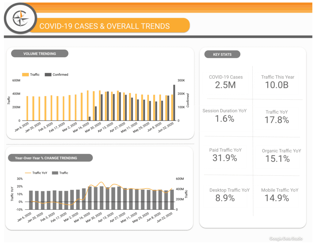
We want to create a dashboard that shows the number of sessions, pageviews, transactions, and goals that took place in the last hour. In the same visualization, we want the same measurements of the same hour of yesterday and a week ago.
Google Analytics Real-Time Reporting
The real-time reports built into Google Analytics are very useful for checking some real-time metrics and verifying event implementation and goal configuration, among other benefits. The real-time reporting that we’re configuring in this blog post will include additional metrics – eCommerce transactions specifically – and will also provide date comparisons and different time-series visualizations.
As for the measurements from yesterday and from a week ago, we can get them from the finalized daily tables. We should always remember that data from the continuous export is from live sessions that are still running and that all of the session totals are not final.
In planning and design, we start from the end goal and move backwards:
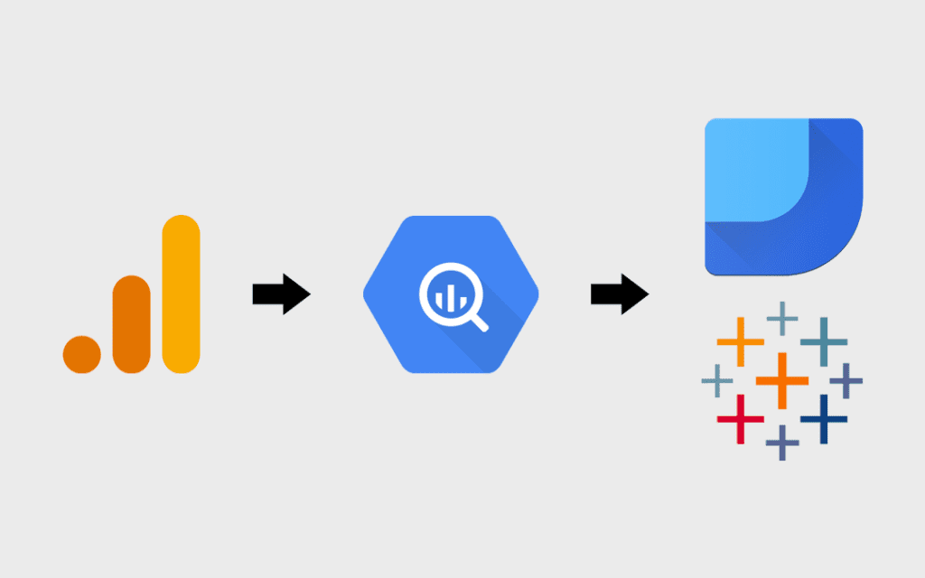
- We design the dashboard in Data Studio or Tableau, reading data from BigQuery;
- Then we design the intermediate reporting table feeding the visualization;
- Then we design the queries/jobs that will create this intermediate table;
The query and the intermediate table
So, the intermediate table should have the following metrics, in addition to the hour dimension:
| Sessions | Pageviews | Transactions | goal1_completed | |
| From 45 min ago | ||||
| Same hour from yesterday | ||||
| Same hour from a week ago |
We can extend or simplify these metrics. To focus on the workflow, let’s simplify it and only include the number of sessions and pageviews and the data from a week ago.
The query should look like this:
SELECT<br />lastWeek.sessionHour AS sessionHourUTC,<br />IF(lastWeek.sessionHour < 7,lastWeek.sessionHour+17 ,lastWeek.sessionHour-7) AS sessionHourPDT,<br />IFNULL(lastWeekSessions,0) as lastWeekSessions,<br />IFNULL(lastWeekPageviews,0) As lastWeekPageviews,<br />IFNULL(sessions,0) as sessions,<br />IFNULL(pageviews,0) as pageviews, ROUND(100*(IFNULL(sessions,0)-lastWeekSessions)/lastWeekSessions,2) as changeInSessions,<br />ROUND(100*(IFNULL(pageviews,0)-lastWeekPageviews)/lastWeekPageviews,2) as changeInPageviews<br />FROM (<br />SELECT<br />HOUR(TIMESTAMP(INTEGER(visitStartTime*1000000))) AS sessionHour,<br />SUM(IFNULL(totals.visits,0)) AS lastWeekSessions,<br />SUM(IFNULL(totals.pageviews,0)) AS lastWeekPageviews,<br />FROM<br />table_date_range([<project-id>:<dataset-id>.ga_sessions_],<br />DATE_ADD(CURRENT_TIMESTAMP(), -7, "DAY"),<br />DATE_ADD(CURRENT_TIMESTAMP(), -7, "DAY"))<br />GROUP BY<br />sessionHour ) lastWeek<br />LEFT OUTER JOIN (<br />SELECT<br />IFNULL(HOUR(TIMESTAMP(INTEGER(visitStartTime*1000000))),0) AS sessionHour,<br />SUM(IFNULL(totals.visits,0)) AS sessions,<br />SUM(IFNULL(totals.pageviews,0)) AS pageviews,<br />FROM<br />TABLE_DATE_RANGE([<project-id>:<dataset-id>.ga_realtime_sessions_view_], CURRENT_TIMESTAMP(), CURRENT_TIMESTAMP())<br />GROUP BY<br />sessionHour ) today<br />ON<br />lastWeek.sessionHour = today.sessionHour<br />ORDER BY<br />2<br />
- In this query, we assume the local time of the site, as well as the GA View is PDT, that is GMT-7. So, the first column will show hours in UTC and the second column will show the hours in local time. If your website is in a different time zone you would need to change this line of the query.
- We will group the number of sessions and pageviews every hours.
- The query may run at any time of day. Throughout the day, every time it runs, the metrics, i.e. sessions and pageviews, of older hours of the day will be updated with more accurate numbers. The later hours of the day won’t be populated with data until those hours are reached. That is, we used LEFT OUTER JOIN since during the day many hours won’t have any data yet.
During the day, the intermediate table will look like this:

The table is showing the hour of the day, metrics from today, metrics from a week ago, and the percentage of change.
Lag time and Window time
In some cases, the GA data exported to BigQuery is required to feed other systems for other purposes, for example, to feed a specific analysis tool. If you’re exporting the data to another system, you have to use a slightly different approach:
We can run a query that gets us the last hour after a certain delay time. That is, we have to set up our data to suffer purposely from a delay, to give enough time for the majority of the sessions to conclude and have numbers as close as possible to the final numbers. We will refer to this delay as lag time.
Another knob that we have to adjust is the window time. Assuming we will aggregate these measurements every 1 hour, that means our data will have 24 readings every day, every 2 hours leads to 12 readings every day and so on.
Adjusting lag time and Window time.
The best values for lag time and window time are set part in configuration and part in the hard-coded queries. They vary a lot from one site to another. For best results, there is a balance that has to be achieved between two things: achieving minimum lag time, i.e. becoming close to real-time, and the accuracy of the numbers collected. For our experiment, let’s assume a lag time of 30 minutes and a window of 1 hour.
The following table illustrates when our queries will run and the window it covers, for a lag of 30 min and a window of 1 hour:
| Query Run Time (with 30-minute lag time) | Window Start Time | Window End Time |
| 0:30 | 11:00 PM (previous day) | 12:00 AM (midnight) |
| 1:30 AM | 00:00 AM | 1:00 AM |
| 2:30 AM | 1:00 AM | 2:00 AM |
| 3:30 AM | 2:00 AM | 3:00 AM |
| 4:30 AM | 3:00 AM | 4:00 AM |
| 4:30 AM | 3:00 AM | 4:00 AM |
| 5:30 AM | 4:00 AM | 5:00 AM |
| 6:30 AM | 5:00 AM | 6:00 AM |
| 11:30 PM | 10:00 PM | 11:00 PM |
Query run time (with 30-minute lag time) and window time.
From the above schedule, we notice that:
The first job will run against the data of the previous day. Luckily, the real-time table/view doesn’t get flushed away at midnight. If the lag time increases this may apply to the second or the third run as well.
Now, the automation:
There are two very versatile GCP components called Cloud Functions and Cloud Scheduler. Mahmoud Taha, from our data engineering team, has covered them in a previous post, where he explained how to create a workaround for the fact that Cloud Functions cannot be triggered by BigQuery.
Unlike the use case discussed in that previous post, we won’t need Cloud Functions to listen to events raised by BigQuery or Stackdriver; instead, we’ll take advantage of Cloud Scheduler for a timed approach. Specifically, we will configure Cloud Scheduler to invoke a Cloud Function according to the schedule outlined in the table above. The cloud function will run the query against the real-time View and save the output to an intermediate BQ table. As explained earlier, the selected lag time and window time will affect the configuration of the Cloud Scheduler and the query invoked by the Cloud Function. The cloud function will always overwrite the intermediate table, making the latest measurements available to the visualization tool.
Nice thing from Google is that they’ve created libraries in several languages that make writing code to interact with APIs of GCP component, such as BigQuery, a breeze. Here is the code that we can include in a Google Cloud Function to invoke the above-mentioned query and to save the result as an intermediate table, overwriting the old data.
from google.cloud import bigquery<br />from datetime import datetime</p><p>bq_tables_dataset = "<dataset-id>"<br />bq_query = """ SELECT<br />lastWeek.sessionHour AS sessionHourUTC,<br />IF(lastWeek.sessionHour < 7,lastWeek.sessionHour+17 ,lastWeek.sessionHour-7) AS sessionHourPDT,<br />IFNULL(lastWeekSessions,0) as lastWeekSessions,<br />IFNULL(lastWeekPageviews,0) As lastWeekPageviews,<br />IFNULL(sessions,0) as sessions,<br />IFNULL(pageviews,0) as pageviews,<br />ROUND(100*(IFNULL(sessions,0)-lastWeekSessions)/lastWeekSessions,2) as changeInSessions,<br />ROUND(100*(IFNULL(pageviews,0)-lastWeekPageviews)/lastWeekPageviews,2) as changeInPageviews<br />FROM (<br />SELECT<br />HOUR(TIMESTAMP(INTEGER(visitStartTime*1000000))) AS sessionHour,<br />SUM(IFNULL(totals.visits,0)) AS lastWeekSessions,<br />SUM(IFNULL(totals.pageviews,0)) AS lastWeekPageviews<br />FROM<br />table_date_range([<project-id>:<dataset-id>.ga_sessions_],<br />DATE_ADD(CURRENT_TIMESTAMP(), -7, 'DAY'),<br />DATE_ADD(CURRENT_TIMESTAMP(), -7, 'DAY'))<br />GROUP BY<br />sessionHour ) lastWeek<br />LEFT OUTER JOIN (<br />SELECT<br />IFNULL(HOUR(TIMESTAMP(INTEGER(visitStartTime*1000000))),0) AS sessionHour,<br />SUM(IFNULL(totals.visits,0)) AS sessions,<br />SUM(IFNULL(totals.pageviews,0)) AS pageviews,<br />FROM TABLE_DATE_RANGE([<project-id>:<dataset-id>.ga_realtime_sessions_view_], CURRENT_TIMESTAMP(), CURRENT_TIMESTAMP())<br />GROUP BY<br />sessionHour ) today<br />ON<br />lastWeek.sessionHour = today.sessionHour<br />ORDER BY<br />2<br />"""</p><p>#entry point for HTTP triggered Cloud Function<br />def save_to_bq(request):<br />bq_client = bigquery.Client()<br />executionDay = datetime.now().strftime('%Y%m%d')<br />executionHour = datetime.now().strftime('%H')</p><p># Saving data to an intermediate table in BQ<br />bq_table_name = 'TableName_{}_{}'.format(executionDay,executionHour)<br /># execute<br />run_query_job(bq_client, bq_query, bq_table_name)</p><p># exit function<br />return 'Done!'</p><p>def run_query_job(bq_client, query, tableId):<br />job_config = bigquery.QueryJobConfig()<br /># Set the destination table<br />table_ref = bq_client.dataset(bq_tables_dataset).table(tableId)<br />job_config.destination = table_ref<br />job_config.allow_large_results = True<br />job_config.use_legacy_sql = True<br />job_config.write_disposition = 'WRITE_TRUNCATE'</p><p># Start the query, passing in the extra configuration.<br />query_job = bq_client.query(<br />query,<br />location='US', # should match project's location<br />job_config=job_config) # API request - starts the query</p><p>query_job.result() # Waits for the query to finish<br />Python code for the cloud function that updates an intermediate table in BigQuery based on real-time GA table/view in BigQuery.
Let’s say, we will configure Cloud Scheduler to invoke Cloud Functions and run this code every 15-30 minutes, updating/overwriting the intermediate table. This setup will make the intermediate table act as a caching mechanism, instead of running the queries every time the dashboard is displayed.
Tying Cloud Functions and Cloud Scheduler
One of the well-designed features of Cloud Functions is how it can be triggered. That is, through HTTP, Cloud Storage, Cloud PubSub, and several Firebase components.
Support for HTTP makes it easy to create web hooks and integrate it with several apps beyond GCP. Here, we are interested in hooking it with a GCP component; namely Cloud Scheduler.
Once we choose a name for our function and HTTP as our trigger, a URL will be displayed. That’s what we will use in Cloud Scheduler.

Configuring Cloud Scheduler
Configuration of Cloud Scheduler is straightforward, maybe with one exception; the frequency. Here is Google’s documentation on how to configure the frequency.
After determining the proper lag time and window time and creating the time table above, we can adjust the query invoked by Cloud Functions and the frequency of making the HTTP calls by the Cloud Scheduler. The time table makes it much simpler than working these adjustments in one’s head.

Once we choose HTTP as a target, more details will appear:

This is where we enter the URL we got from Cloud Functions. And that’s it. Cloud Scheduler will invoke the Cloud Function, the Cloud Function will run the query and save the output to the intermediate table and make it available to the visualization tool.
Caveat:
The biggest caveat we noticed in our testing/implementation is that, sometimes, the numbers go really low compared to last week, apparently due to high hit traffic. This is not a real drop; it’s just a delay in processing the hits and exporting it from GA 360 to BigQuery. That is just the nature of streaming data asynchronously; no one cannot guarantee when the streaming data will arrive or in what order. In many cases, this has been solved by increasing the lag time whenever the business allowed for that.
Improvements
First, we don’t have to worry about the automation and using Cloud Functions/Cloud Scheduler if our visualization tool can run the query periodically and cache the result. Several visualization tools have this capability.
Second, we notice that we calculate the metrics for the historical data, i.e. from yesterday and from a week ago, every time we run the query that updates the reporting table. This step can also be automated and scheduled to run once a day and save the result to another intermediate table, let’s call it historical_metrics_by_hour. Our first query has to be rewritten to read from this table and from the real-time BQ View to update the reporting table. The extra work involved improves performance and cost. It’s your call to keep it simple or to keep it efficient. It varies from one case to another.
Summary:
Real-time export of GA 360 data into BigQuery is a great feature. One has to find a balance between data freshness and data completeness. There are several GCP components that can be integrated to create several useful dashboards and alerts systems. All we have to do is to configure and hook these components together and we would have a cloud-based solution. If you have other ideas or similar use cases, please leave a comment.
Resources
- https://support.google.com/analytics/answer/7430726?hl=en
- https://support.google.com/analytics/answer/7084038
- https://cloud.google.com/functions/docs/
- https://cloud.google.com/scheduler/docs/
- https://www.cardinalpath.com/blog/cloud-functions-bigquery-data-feed-automation